Python has established itself as the go-to programming language in the field of data science. However, Microsoft Excel remains a popular and easy-to-use tool for conducting data analysis or presenting information to stakeholders. Excel’s prevalence in the business world, along with its familiar interface, makes it a valuable resource for generating analysis and reports that need to be shared with other departments within an organization.
Microsoft Excel is one of the most widely used spreadsheet software in the world, offering a comprehensive set of features and tools to help professionals analyze, organize, and present data. Among its vast array of functions, there are a few that stand out as essential for data analysts looking to streamline their workflow and improve their productivity.
With over 500 functions available in Excel, it can be daunting to know where to start when it comes to data analysis. It can be difficult to determine which functions are best suited for specific tasks, given the extensive range of options available.
The most useful Excel functions are the ones that make your job seem effortless. The good news is that most Excel users have a set of reliable functions that can perform the majority of their needs.
By the end of this article, you’ll have an understanding of the basic and most common functions of Excel used by Data Analysts, Data Scientists and other professionals who work on data, with an appreciation for its capabilities.
We will discuss Top 14 of the most useful Excel functions that can boost your data analysis productivity and help you perform common data analyst tasks quickly and efficiently.
Most Common Excel Functions used by Data Analysts
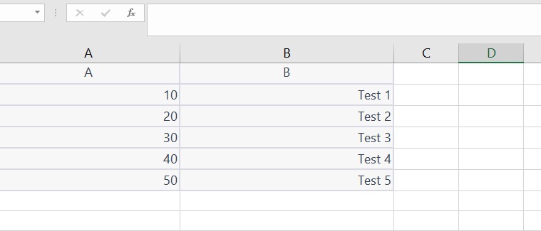
Let’s take an example Excel Sheet that demonstrates the usage of the functions:

- SUM Function:
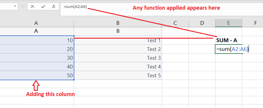
The SUM function adds up a range of values in a worksheet. To use it, follow these steps:
Step 1: Select the cell where you want the result to appear.
Step 2: Type the following formula: =SUM(range), where “range” is the range of cells you want to add.
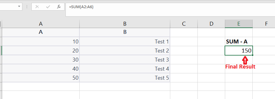
For example, to add the values in cells A1 to A5, you would type =SUM(A1:A5).
Suppose you have a list of numbers in cells A1 to A5, and you want to add them up. You can use the SUM function like this:
=SUM(A1:A5)
This will give you the sum of the numbers in cells A1 to A5.


- AVERAGE Function:
The AVERAGE function calculates the average of a range of values in a worksheet. To use it, follow these steps:
Step 1: Select the cell where you want the result to appear.
Step 2: Type the following formula: =AVERAGE(range), where “range” is the range of cells you want to average.
For example, to average the values in cells A1 to A5, you would type =AVERAGE(A1:A5).
To find the average of the test scores in Column A (Refer above sheet), you can use the AVERAGE function like this:
=AVERAGE(A1:A5)
The result will be 30.
- COUNT Function:
The COUNT function counts the number of cells in a range that contain numeric values. To use it, follow these steps:
Step 1: Select the cell where you want the result to appear.
Step 2: Type the following formula: =COUNT(range), where “range” is the range of cells you want to count.
For example, to count the number of cells in cells A1 to A5 that contain numeric values, you would type =COUNT(A1:A5).
To count the number of tests in Column B (Refer above sheet), you can use the COUNT function like this:
=COUNT(B1:B5)
The result will be 5.
- MAX Function:
The MAX function returns the highest value in a range of cells. To use it, follow these steps:
Step 1: Select the cell where you want the result to appear.
Step 2: Type the following formula: =MAX(range), where “range” is the range of cells you want to find the maximum value.
For example, to find the highest value in cells A1 to A5, you would type =MAX(A1:A5).
To find the highest and lowest test scores in Column A (Refer above sheet), you can use the MAX function like this:
=MAX(A1:A5)
The result will be 50.
These will give you the highest test scores, respectively.
- MIN Function:
The MIN function returns the lowest value in a range of cells. To use it, follow these steps:
Step 1: Select the cell where you want the result to appear.
Step 2: Type the following formula: =MIN(range), where “range” is the range of cells you want to find the minimum value.
For example, to find the lowest value in cells A1 to A5 (Refer above sheet), you would type =MIN(A1:A5).
=MIN(A1:A5)
The result will be 10.
These will give you the lowest test scores, respectively.
- IF Function:
The IF function allows you to test a condition and return one value if the condition is true, and another value if the condition is false. To use it, follow these steps:
Step 1: Select the cell where you want the result to appear.
Step 2: Type the following formula: =IF(condition, value_if_true, value_if_false), where “condition” is the condition you want to test, “value_if_true” is the value you want to return if the condition is true, and “value_if_false” is the value you want to return if the condition is false.
For example, if you want to test if the value in cell A1 is greater than 10 and return “Yes” if it is, and “No” if it’s not, you would type =IF(A1>10,”Yes”,”No”).
To categorize the test scores in Column A (Refer above sheet) as “pass” or “fail” based on a passing score of 25, you can use the IF function like this:
=IF(A1>=25,"Pass","Fail")
The result will be “Fail” for cell A1 and A2, “Pass” for cells A3 to A5.
- VLOOKUP Function:
The VLOOKUP function searches for a value in the first column of a table and returns a value in the same row from a specified column. To use it, follow these steps:
Step 1: Select the cell where you want the result to appear.
Step 2: Type the following formula: =VLOOKUP(lookup_value, table_array, column_index_num, [range_lookup]), where “lookup_value” is the value you want to search for, “table_array” is the range of cells that contain the table you want to search in, “column_index_num” is the column number in the table that contains the value you want to return, and “range_lookup” is an optional argument that specifies whether you want an exact match or an approximate match.
For example, if you have a table that lists the names of employees in column A and their salaries in column B, and you want to look up the salary of an employee whose name is in cell C1, you would type =VLOOKUP(C1,A:B,2,FALSE). This would return the salary of the employee in cell C1.
Suppose you have a table of employee names and salaries in cells A1 to B5, and you want to look up the salary of a particular employee whose name is in cell C1. You can use the VLOOKUP function like this:
=VLOOKUP(C1,A1:B5,2,FALSE)
This will look up the name in cell C1 in the first column of the table (A1:A5), and return the corresponding salary from the second column (B1:B5). Or
To look up the salary of an employee named “Alice” in a table of employee names and salaries in cells A1 to B5, you can use the VLOOKUP function like this:
=VLOOKUP("Alice",A1:B5,2,FALSE)
Assuming that “Alice” is in cell C1, the result will be the salary of the employee named Alice in the second column of the table (Column B).
=> Let’s see this with help of an Excel Sheet –
| Employee Name | Salary |
|---|---|
| Alice | 50000 |
| Bob | 60000 |
| Charlie | 55000 |
| David | 65000 |
| Emma | 70000 |
- In cell C1, type “Alice” to indicate the employee name you want to look up.
- In cell D1, enter the VLOOKUP formula =VLOOKUP(C1,A1:B5,2,FALSE).
- The result will be the salary of the employee named Alice in the second column of the table (Column B), which is 50000. The Excel sheet should now look like this:
| Employee Name | Salary | C | D |
|---|---|---|---|
| Alice | 50000 | Alice | 50000 |
| Bob | 60000 | ||
| Charlie | 55000 | ||
| David | 65000 | ||
| Emma | 70000 |
- CONCATENATE Function:
The CONCATENATE function allows you to join two or more text strings into one string. To use it, follow these steps:
Step 1: Select the cell where you want the result to appear.
Step 2: Type the following formula: =CONCATENATE(text1, [text2], …), where “text1”, “text2”, etc. are the text strings you want to join.
For example, if you want to join the text strings “John” and “Doe” into one string, you would type =CONCATENATE(“John”, “Doe”). This would return the string “JohnDoe”.
To join the first name in cell A1 and the last name in cell B1 into a full name, you can use the CONCATENATE function like this:
=CONCATENATE(A1," ",B1)
The result will be “John Smith” assuming that “John” is in cell A1 and “Smith” is in cell B1.
- LEFT and RIGHT Functions:
The LEFT and RIGHT functions allow you to extract characters from the beginning or end of a text string. To use them, follow these steps:
Step 1: Select the cell where you want the result to appear.
Step 2: Type the following formula for LEFT: =LEFT(text, [num_chars]), where “text” is the text string you want to extract characters from, and “num_chars” is the number of characters you want to extract from the beginning of the string.
Step 2: Type the following formula for RIGHT: =RIGHT(text, [num_chars]), where “text” is the text string you want to extract characters from, and “num_chars” is the number of characters you want to extract from the end of the string.
For example, if you have the text string “Hello World” in cell A1 and you want to extract the first 5 characters, you would type =LEFT(A1,5). This would return the string “Hello”. If you want to extract the last 5 characters instead, you would type =RIGHT(A1,5). This would return the string “World”.
To extract the first three characters from the string “Data Analyst” in cell A1, you can use the LEFT function like this:
=LEFT(A1,3)
The result will be “Dat”.
To extract the last four characters from the same string, you can use the RIGHT function like this:
=RIGHT(A1,4)
The result will be “lyst”.
- TEXT Function:
The TEXT function allows you to convert a value to text in a specified format. To use it, follow these steps:
Step 1: Select the cell where you want the result to appear.
Step 2: Type the following formula: =TEXT(value, format_text), where “value” is the value you want to convert to text, and “format_text” is the format you want to apply to the text.
For example, if you have the value 12345 in cell A1 and you want to convert it to text with a comma separator, you would type =TEXT(A1,”#,###”). This would return the string “12,345”.
Some other Excel common, basic and useful functions
11. LEN Function:
To find the length of the string “Data Analyst” in cell A1, you can use the LEN function like this:
=LEN(A1)
The result will be 12.
12. TRIM Function:
To remove extra spaces from a text string, you can use the TRIM function like this:
=TRIM(" Data Analyst ")
The result will be “Data Analyst” without the extra spaces.
13. DATE Function:
To create a date in Excel, you can use the DATE function. For example, to create the date “May 11, 2023”, you can use this formula:
=DATE(2023,5,11)
The result will be the date in the format “5/11/2023”.
14. TODAY Function:
To get today’s date in Excel, you can use the TODAY function like this:
=TODAY()
The result will be the current date in the format “5/11/2023”.
Conclusion
These are just a few of the most commonly, basic and useful Excel functions used for data analysis, but there are many more functions available depending on your specific needs. To explore and start your career with Excel as a Data Analyst, we recommend this course –

Prabhat Kumar is a Senior Editor at DataBonker, specializing in Education, Career, Admissions, and Technology. With a keen eye for detail and a passion for delivering insightful content, he curates well-researched articles that help readers navigate their academic and professional journeys. From career advice to the latest trends in education and emerging technologies, Prabhat ensures every piece is informative, engaging, and valuable.
📩 **Stay Ahead with DataBonker!**
Join our newsletter and get the latest insights on "Education, Admissions Guidance, Career Growth, Latest Job Trends, and Technology Updates** – straight to your inbox! 🚀
